Creating Your Potential

pele has a number of potentials built in, including the Lennard-Jones potential which is used for most of our examples. It also has an interface to the GMIN program with which you can access any myriad of GMIN’s built in potentials. We also plan to build interfaces to some of the standard molecular dynamics packages like gromacs and OpenMM.

The flexibility of pele alows it to be easily used with just about any scalar function. Probably the biggest limitation is that, because we use a lot of gradient based local minimization you may experience problems if your potential is discontinuous.

simple 1D potential

Lets create an artificial potential from the sum of a parabola and a cosine term:

from pele.potentials import BasePotential
import numpy as np
class My1DPot(BasePotential):
    def getEnergy(x):
        return np.cos(14.5 * x[0] - 0.3) + (x[0] + 0.2) * x[0]

The above definition of member function getEnergy() is all that is required to use the global optimization features of pele. It is derived from BasePotential, which will calculate gradient numerically. However, Defining an analytical gradient will make things run a lot faster:

from pele.potentials import BasePotential
import numpy as np
class My1DPot(BasePotential):
    """1d potential"""
    def getEnergy(self, x):
        return np.cos(14.5 * x[0] - 0.3) + (x[0] + 0.2) * x[0]

    def getEnergyGradient(self, x):
        E = self.getEnergy(x)
        grad = np.array([-14.5 * np.sin(14.5 * x[0] - 0.3) + 2. * x[0] + 0.2])
        return E, grad

From this point you can jump in and use BasinHopping to find the global minimum. The best way to do this is to use the convience wrapper, the system class. As a first start, all we must do is tell the system class what our potential is

from pele.systems import BaseSystem
class My1DSystem(BaseSystem):
    def get_potential(self):
        return My1DPot()

The following code will use the system class to initialize a basinhopping class and run basinhopping for 100 steps. We use an sqlite database to store the minima found:

system = My1DSystem()
database = system.create_database()
x0 = np.array([1.])
bh = system.get_basinhopping(database=database, coords=x0)
bh.run(100)
print "found", len(database.minima()), "minima"
min0 = database.minima()[0]
print "lowest minimum found at", min0.coords, "with energy", min0.energy

atomic pair potential

We now look at a more involved system. Lets create a system of atoms interacting via a pair potential similar to the Lennard-Jones potential. See pele/examples/new_potential/ for the code related to this example:

from pele.potentials import BasePotential
class MyPot(BasePotential):
    """a Lennard Jones potential with altered exponents

    E(r) = r**-24 - r**-12
    """
    def __init__(self, natoms):
        self.natoms = natoms #number of atoms

    def getEnergy(self, coords):
        coords = np.reshape(coords, [natoms,3])
        E = 0.
        for i in range(natoms):
            for j in range(i):
                r = np.sqrt(np.sum((coords[i,:] - coords[j,:])**2))
                E += r**-24 - r**-12
        return E

    def getEnergyGradient(self, coords):
        coords = np.reshape(coords, [natoms,3])
        E = 0.
        grad = np.zeros(coords.shape)
        for i in range(natoms):
            for j in range(i):
                dr = coords[i,:] - coords[j,:]
                r = np.sqrt(np.sum(dr**2))
                E += r**(-24) - r**(-12)
                g = 24. * r**(-25) - 12. * r**(-13)
                grad[i,:] += -g * dr/r
                grad[j,:] += g * dr/r
        return E, grad.reshape(-1)

We have getEnergy and getEnergyGradient implemented, so the potential is ready to use.

Tip

Loops in python are very slow. The above functions getEnergy() and getEnergyGradient() will run a lot faster in a compiled language. Good choices might be cython or c++ wrapped with cython. See the included potential pele.potentials.LJ for an example of how to do this.

We are now ready to define the system class.

from pele.systems import BaseSystem
class MySystem(BaseSystem):
    def __init__(self, natoms):
        super(MySystem, self).__init__()
        self.natoms = natoms
        self.params.database.accuracy = 0.001

    def get_potential(self):
        return MyPot(self.natoms)

We can now run basinhopping in exactly the same way we did before:

import numpy as np
natoms = 8
system = MySystem(natoms)
database = system.create_database()
x0 = np.random.uniform(-1,1,[natoms*3])
bh = system.get_basinhopping(database=database, coords=x0)
bh.run(10)
print "found", len(database.minima()), "minima"
min0 = database.minima()[0]
print "lowest minimum found has energy", min0.energy

Note

The database (Database) saves all unique minima found, and determines uniqueness through an energy criterion. If two minima have energies closer than database.accuracy then they are deemed to be the same minimum and one is discarded. It might be a good idea to change this accuracy parameter to be more appropriate for your system. This is done in the above example where we set self.params.database.accuracy in __init__(). Note that this must be done after calling the base class __init__().

Distinguishing minima by energy is good, but often not good enough. If you define the function MySystem.get_compare_exact() (which overloads BaseSystem.get_compare_exact()), then the database will use that function in addition to the energy criterion to compare minima. See structure alignment for how to set that up.

Note

One of the core routines of basinhopping is the takestep routine. This is the routine which randomly moves the configuration through phase space. The default is a random displacement of the coordinates where both the step size and the temperature are adaptively adjusted to give the best results. For more complex systems there is often a better way to search. Improving takestep is probably the most important thing you can do to improve the speed at which you find the global minimum. See the global optimization page for more information about how to use alternative, already implemented, takestep routines, and for more information about how to implement your own. If you do choose to use a non-default takestep, you should define MySystem.get_takestep(), which overload BaseSystem.get_takestep() in order to use it with the system class.

finding transition state pathways

We have, to this point, defined a potential, MyPotential, and a system class MySystem with one function get_potential(). This was enough to run basinhopping, but unfortunately is not enough to find transition states and build up the connected network. A few additional functions are required.

Many of the routines in DoubleEndedConnect need a distance metric which returns how far apart are two structures. This is know as mindist (or minpermdist, or structural alignment). We use as our metric the root mean squared deviation, so in the simplest case the mindist function should just be

import numpy as np
def simple_mindist(x1, x2):
    distance = np.linalg.norm(x1 - x2)
    return distance, x1, x2

This functional format, where the distance is returned as well as x1 and x2, is the default for all mindist routines. The simple case breaks down, however, when there are global symmetries of the system. Imagine the system is translationally invariant and X2 is exactly the same as X1, but just translated. Then the root mean squared deviation would give a large distance when the distance should be zero. Thus the distance routine must take into account all the symmetries of a system. Some common symmetries are

1. translational invariance
2. rotational invariance
3. reflection symmetry
4. permutational invariance

pele has all the utilities necessary for handling these cases, but they are, by definition, system dependent, so you must manually specify them for your system. These should be implemented in the system class by overloading MySystem.get_mindist(). See Structure Alignment for how more detailed information and help choosing which routine to use.

Lets continue defining the system class for MyPotential. Lets set it up as a cluster of atoms floating in a vacuum. Thus we have all three spatial symmetries listed above. Assuming the atoms are indistinguishable we also have permutational symmetry. The mindist class which deals with these 4 symmetries is MinPermDistAtomicCluster:

from pele.mindist import MinPermDistAtomicCluster
class MySystem(BaseSystem):
  ...
  def get_mindist(self):
      permlist = [range(self.natoms)]
      return MinPermDistAtomicCluster(permlist=permlist, niter=10)

We’re not quite ready yet. The routine which searches for transition states (FindTransitionState) uses a routine which walks uphill in the direction of the lowest eigenvector (the eigenvector with the lowest eigenvalue) while walking downhill in all other directions. We find this lowest eigenvector by looking for the direction with the largest negative curvature with FindLowestEigenVector. This search is a lot easier and less error prone if the search space is reduced and made simpler by removing the trivial zero eigenvectors. These are directions in phase space which have zero eigenvalue and correspond to trivial global symmetries of the system, e.g. translational and rotational symmetry, or frozen degrees of freedom. In order to implement this, MySystem.get_orthogonalize_to_zero_eigenvectors() must return a function which makes a given vector orthogonal to all trivial zero eigenvectors. See BaseSystem.MySystem.get_orthogonalize_to_zero_eigenvectors() and transition state search for more information. If your system has no zero eigenvalues, that function can just return None. For our cluster system we have 3 zero eigenvectors for translational symmetries and 3 zero eigenvectors for rotational symmetries. The routine which takes care of this is called orthogopt()

from pele.transition_states import orthogopt
class MySystem(BaseSystem):
    ...
    def get_orthogonalize_to_zero_eigenvectors(self):
        return orthogopt

We are now ready to find transition state pathways between minima. As a starting point we will use the database that we built up from the basinhopping run above. We will connect all minima to the lowest energy minimum.

from pele.landscape import ConnectManager
manager = ConnectManager(database, strategy="gmin")
for i in xrange(database.number_of_minima()-1):
    min1, min2 = manager.get_connect_job()
    connect = system.get_double_ended_connect(min1, min2, database)
    connect.connect()

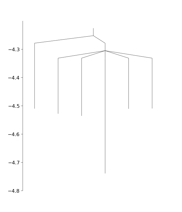
In the above we have used the class ConnectManager to manage which minima pairs to try to connect next. This class has several different strategies for connecting the minima. We now have a fully connected database (though the basinhopping run was quite short, so we may not have found the global minimum yet). As a final step, let’s plot the connectivity in the database using a disconnectivity graph

from pele.utils.disconnectivity_graph import DisconnectivityGraph, database2graph
import matplotlib.pyplot as plt
#convert the database to a networkx graph
graph = database2graph(database)
dg = DisconnectivityGraph(graph, nlevels=3, center_gmin=True)
dg.calculate()
dg.plot()
plt.show()